Presentation of the Open Trade Project
Understand our data-driven grading approach
Welcome to the Open Trade Project!
I’ve always been interested in data analysis and how it applies to the roster building aspects of NFL teams, and draft season is one of my favorite parts of the year. The league is increasingly paying attention to data science, as evidenced by NFL Next Gen Stats and Pro Football Focus. The internet is full of mock drafts and projections and I wanted to contribute in some way.
Scouting prospects is a highly subjective process; each team has its own priorities and athletic requirements, and we’ll never know what happens inside war rooms. I wanted to stay away from speculating and projecting players as much as possible. Eventually, I had an idea: how to reimagine the current NFL trade chart using modern data analysis techniques? The result is The Open Trade Project.
Over the past few months, I have gathered data for all NFL draft trades since 2002 (when the current format was established). I evaluated the trades using the classic Jimmy Johnson model and added uncertainty to the value of each pick using machine learning. I also developed an open, free-to-use draft trade grader.
This post is an overview of the project, or “the very minimum that you need to know” if you want to use this model. In the upcoming weeks, further posts will take a deep dive on specific aspects.
Trades for the 2025 NFL Draft will be graded live here.
The Jimmy Johnson trade chart
The Jimmy Johnson Trade Value Chart is a widely used tool in the NFL to assess the relative value of draft picks during trades. Created in the early 1990s by former Dallas Cowboys head coach Jimmy Johnson, the chart assigns a numerical value to each pick in the draft, with the highest values placed on early first-round selections and progressively lower values assigned to later picks. This straightforward scoring system helps teams evaluate whether a proposed trade involving draft picks is fair or advantageous.
 The classic Jimmy Johnson Trade Value Chart, a staple in NFL draft trade analysis. The value function decays very rapidly.
NFL draft trades don’t always reflect pick values according to the Jimmy Johnson model, leading to speculation about “winners or losers” for each trade, as well as the creation of new models which better describe more recent trades, such as the Rich Hill model. There is a common aspect in both models: each pick has a fixed value; for example, pick 21 is worth 800 points in the Jimmy Johnson chart. Suppose 3 hypothetical trades, where pick 21 sells for 780, 800 and 820 points. On average, pick 21 was transacted for 800 points. But how about the variance?
No love for standard deviation?
Suppose the average cost of a gallon of gas in Texas is $2.75. That does not mean that every gallon of gas in Texas sells for that much. In fact, there is a variability of gas prices around the mean; that variability is called standard deviation. Suppose that, in our example, the standard deviation is 10 cents. If the price distribution is normal, according to the theory of normal distributions, 68% of the gallons of gas in Texas are sold for an amount between $2.65 and $2.85; 95% are sold for an amount between $2.55 and $2.95; and 99% are sold for an amount between $2.45 and $3.05.
This example provides a valuable takeaway in terms of evaluating draft charts. Both options describe the value of picks only in terms of a mean value; in other words, the possibility of variation in the cost due to external circumstances is disregarded. In the real NFL draft, multiple factors affect the value of a pick, just like the cost of gas across different gas stations. It is clear that any redesign of the Jimmy Johnson model that does not take cost variability into account will not capture all the information that the available data on past trades has to offer.
Including variability in the cost of draft picks
Our goal is to fit a normal distribution for each pick, so that, instead of saying “pick 21 is worth 800 points”, we will say (for example) “the value for pick 21 has a mean of 800 points and a standard deviation of 28 points”. The second statement carries much more information: using the same approach as in the gas example, we can say that, in 68% of trades, pick 21 sells for between 772 and 828 points; in 95% of the trades, it sells for between 744 and 856 points; and, in 99% of the trades, it sells for between 716 and 894 points. For most real world applications, the interval corresponding to 95% of the transactions is considered “normal” or “typical”. This means that, in our case, pick 21 is reasonably expected to sell for a value between 744 and 856 points.
How to determine the cost variability for each pick?
The possibility of calculating mean and standard deviation presents a great opportunity for the development of a more accurate draft chart. In the drafts between 2002 and 2024, there has been a great number of trades. The starting dataset constitutes of these trades, and presents a few challenges:
- Trades mostly involve multiple picks being transacted, making it hard to pinpoint the value that each pick is selling for. For example, if a team ships picks 21 and 144 for picks worth 850 points, part of that value is being paid for pick 21 and part is being paid for pick 144. The strategy to deal with that challenge will be presented in an upcoming post.
- Many trades involve players. The goal of this project is to evaluate the value of picks, so a choice was made to disconsider trades involving players, regardless of whether the player is a future hall of famer or a borderline starter.
- Many trades also involve future picks, increasing the uncertainty (since not all picks are known at the time of the trade). For now, the model does not support trades involving future picks, although a future evolution certainly will be able to handle that scenario.
These limitations reduce our dataset to 453 observed trades (down from 561 if future picks are considered). Each of these trades was recorded in a text file. One example is shown below:
2023 DET “6;81” ARI “12;34;168” D
In that example, Detroit traded picks 6 and 81 to Arizona, receiving picks 12, 34 and 168 in return.
Once all trades were compiled, the value for each trade was calculated by means of the Jimmy Johnson chart. In our previous example, Detroit received 1785 points, while Arizona received 1784.2 points. These calculations provide many insights, to be explored in a future post. For now, it is enough to state that the Jimmy Johnson trade chart is not as bad as people think, as far as the average value of each pick is concerned.
The mathematical model
For simplicity (and according to the observations of the previous paragraph), it was assumed that the average value for each pick provided by the Jimmy Johnson trade chart is correct. The model focuses on the variability, i.e., the accepted uncertainty around that value. The detailed description of the model is highly mathematical and may not be of interest to every reader, and will be provided in a separate post.
In very simple terms, we are assuming that the value of each pick is normally distributed, with the average value provided by the Jimmy Johnson chart. Then, we are applying an artificial intelligence model to determine the standard deviation for each pick. A standard deviation of 28 points for pick 21 is an actual output of our model; as another example, pick 91 has an average value of 136 points and a standard deviation of 11.6 points. The model was fine-tuned to account for further challenges.
For example, none of the 453 trades in the dataset involve pick 1. In that case, we considered that trades involving the surrounding picks (for example, picks 2, 3 and 4) affect the value of pick 1, each to a different extent (a trade involving pick 2 affects the value of pick 1 more than a trade involving pick 3 affects the value of pick 1, for example). This approach makes extensive use of correlation theory and was useful for other picks when data was lacking.
The AI model outputs standard deviations for each pick. That information enables the creation of the most user-friendly feature of the project. The draft simulator.
Grading: a natural evolution of variability analysis
After the mean and standard deviation are known, it is possible to take advantage of another cool feature of normal distributions: percentiles. For example, if a team sells pick 21 for 836 points, they got a 90-th percentile value (better value than 90% of all trades involving that pick). Similarly, the 10-th percentile value (bottom 10% value among all possible trades) is 764 points. Percentiles are really useful when it comes to grading transactions (but, as we’ll see, considering only percentiles is not always a fair way to evaluate trades).
The draft grade simulator
The visual output of the Open Trade Project is a draft simulator/grader, available here. Simply choose the team identifiers and enter pick numbers, and the simulator will generate a card featuring information about the trade and color-coded grades. The cards are free to use and share!
The grading algorithm
Let’s exemplify how the trading algorithm works with a trade from 2022. The Packers traded up for WR Christian Waston, surrending picks 53 and 59 to the Vikings in exchange for pick 34:
In 2022, the Packers traded up for WR Christian Watson. According to the Jimmy Johnson chart, the Vikings surrendered 560 points and received 680 points. https://t.co/qoTAeq5WRd pic.twitter.com/rYwihsJw9X
— The Open Trade Project (@TheOpenTrade) March 31, 2025
In this trade, Minnesota gained a whopping 120 points. Likewise, Green Bay lost 120 points. Considering the Jimmy Johnson trade chart, this was obviously a good trade for Minnesota; according to our model, Minnesota got a 99-plus percentile value for its pick; Green Bay got less than a 1-percentile value.
Minnesota’s grade reflects one of our grading parameters: value. If a team gets a high percentile value on a trade, its grade will always at least match that number (and will be potentially higher).
On the other hand, it seems that Green Bay still got a decent grade, despite getting a bad percentile value on the trade. Our grading model includes additional parameters to make grading more fair on certain conditions. In that case, Green Bay is trading up 19 picks in the second round. It is understood that the team trading up will likely need to pay a higher price the higher the distance is; therefore, a distance parameter is included. Green Bay’s grade of 55.0 is pretty close to the expected average of 50. This grade is dominated by the distance parameter, and not by the value parameter.
In the previous case, the distance parameter helped the grade of the buyer team; sometimes, it may help the seller team. Here’s an example:
In 2024, the Vikings traded up for QB J.J. McCarthy. According to the Jimmy Johnson chart, the Jets surrended 1309 points and received 1321.6 points. https://t.co/qoTAeq5WRd pic.twitter.com/R8k9qyyu7z
— The Open Trade Project (@TheOpenTrade) March 31, 2025
The value parameter is somewhat balanced: according to our model, New York got a 58-th percentile value and Minnesota got a 42-th percentile value. New York is trading down a single pick; in that case, it is reasonable to assume the team has similarly graded players available. Trading down a just a few picks (one in that case) is assumed to be advantageous to the team trading back. New York gets a combined benefit from the value parameter and the distance parameter, resulting in a grade higher than both; The distance parameter also helps Minnesota’s grade, which is higher than it would be considering only the value parameter.
Lastly, there is a parameter to boost the grades as the pick number increases. As the quality of players available decreases across the rounds, teams have more “equally good” players to choose from, especially in the later rounds. The round parameter was designed to generate more lenient grading for the late rounds.
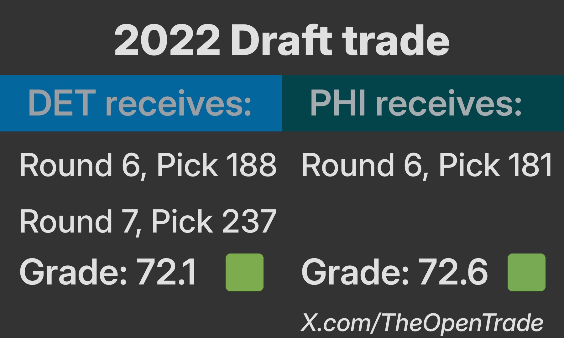 In trades for late round picks, grades are always generous to both teams.
Overall, the grade is always dominated by the highest of the three parameters. The other two parameters only increase the grade. The grading algorithm is complex and will be explored further in a future post.